Official Analysis (C++)

Explanation

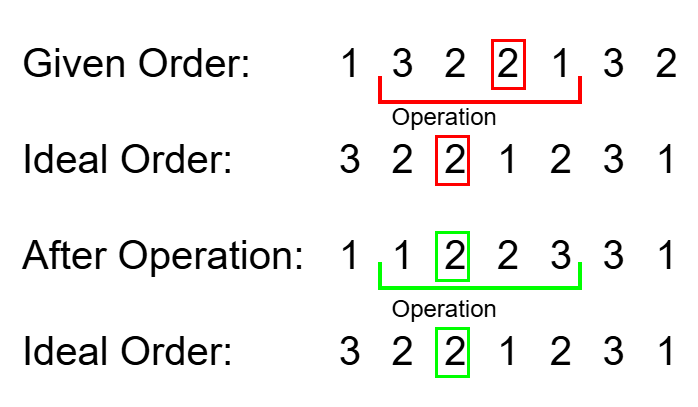
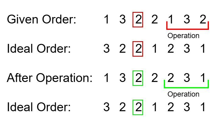
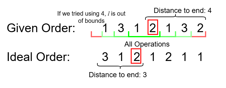
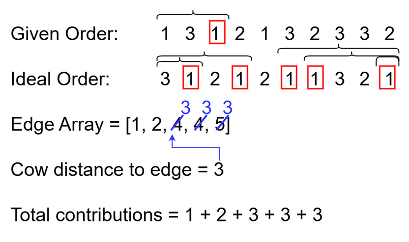
Let's analyze the last test case in detail.

We denote a "desirable location" of a cow as a location where a cow of that species will be checked by the bovine veterinarian.

We denote a "contribution" as one instance of a cow being moved to a desirable location.

Note that a contribution can only be achieved in one of two ways.

The first way is if a cow was not in a desirable location, and the cow was moved to a desirable location during an operation.

The second way is if a cow was already in a desirable location, and the cow was not moved during an operation.

Let's consider how to calculate the contributions created strictly by the first scenario.

Let a cow at location $i$ try to reach a desirable location at location $j$, where $i < j$.

The most intuitive way to achieve this is by setting $l$ to $i$ and $r$ to $j$, so that after the operation, $i$ is moved to $j$.

We observe that the same is true if we set $l$ to $i - 1$ and $r$ to $j + 1$.

Thus, the amount of contributions that can be made from a cow at location $i$ and desirable location at location $j$ is limited by the minimum distance to either end of the order, as after that $l$ or $r$ would violate the given constraints for a valid operation.

In a 0-indexing system, the contribution from $i$ and $j$ can be written as $\min(i + 1, n - j)$.

Now we consider how to calculate contributions created strictly by the second scenario.

Let a cow at position $i$ already be at a desirable location.

The amount of contributions created is equal to the number of operations that do not involve $i$. In the problem, we are given that the number of operations that can occur between $1$ and $N$ can be written as

Thus, the amount of contributions created from a cow at location $i$ at a desirable location can be written as the sum of all the possible operations before and after $i$:

We can implement this by iterating through each cow to determine how many contributions each cow in the initial order makes.

As each cow either is or isn't already at a desirable location, the second scenario is handled with a simple check if the cow is in a desirable location, then applying the formula described above.

However, for the first scenario, there may be multiple desirable locations a cow could move to.

Let's denote a cow and a desirable location that can create contributions as described in the first scenario as a pair $(i, j)$.

If we naively checked each pair, this would take $\mathcal{O}(N)$ time per cow, as in the worst case scenario, each pair of locations is viable.

Let's denote a desirable location's minimum distance to an end as $d_{des}$ and a cow's minimum distance to an end as $d_{cow}$, where $i$ denotes the cow's location and $j$ denotes the desired location.

For a given cow, consider all desirable locations that it can pair with. Each pair contributes $\min(d_{cow}, d_{des})$ contributions. Thus, to speed up processing, we want to separate the pairs which the given cow is a part of into two groups: ones where contributions are limited by $d_{des}$ because $d_{des} < d_{cow}$, and ones where contributions are limited by $d_{cow}$ because $d_{cow} < d_{des}$. We can partition them by creating a sorted array of all $d_{des}$, then binary searching over this array to determine the index where $d_{des} \geq d_{cow}$. Before this index, contributions will be limited by $d_{des}$, and after this index, contributions will be limited by $d_{cow}$.

However, this still results in $\mathcal{O}(N)$ time, since we still have to sum up all $d_{des}$ contributions at the end.

We can optimize this by implementing a prefix sum array that sums the indices $[0, i]$ of the $d_{des}$ array, so we can find the sum of valid $d_{des}$ from the start of a list to any point in $\mathcal{O}(1)$ time. Then, all contributions limited by $d_{cow}$ can be found by multiplying $d_{cow}$ by the number of pairs limited.

Thus, the formula for the contributions provided by the first scenario can be found as written below, given $m$ is the point where $d_{cow}$ becomes less than $d_{des}$:

Implementation

Time Complexity: $\mathcal{O}(N \log N)$

Copy
#include <bits/stdc++.h>
using namespace std;

int main() {
	ios::sync_with_stdio(0);
	cin.tie(0);

	int num_cows;
	cin >> num_cows;

Copy
import bisect

num_cows = int(input())
initial_order = [int(x) for x in input().split()]
ideal_order = [int(x) for x in input().split()]

# Map a cow's species to an array of minimum distances to the edge for that species in the ideal ordering
edge_arrays = dict()

for i in range(num_cows):